Tips and Tricks: Images in cells

As we mentioned a couple of weeks ago, you can now insert images into a cell. With the image() formula you can link to a publicly accessible image and control how it will look with optional parameters. This is useful for bringing a visual element to your spreadsheets for things such as a product catalog listing.

For example the formula
=image("http://www.google.com/intl/en_ALL/images/srpr/logo1w.png", 1) will scale the image down in the current cell. With other parameters you can choose from a variety of sizing options including size to fit, stretch, original size, and even specify a custom size.

Try them all out using this template and let us know what you think in the comments.

Posted by: Li-Wei Lee, Senior Software Engineer

Tips & Tricks: Creating new Google Docs from your mobile

Yesterday, we announced mobile editing on Google Docs, which we've now rolled out to all English-language users.

One of the new features that launched is creating new documents and spreadsheets on your phone. This is particularly useful to jot down quick notes on the run, whether it’s capturing that game-changing idea for your company while at the gym, or typing out your grocery list on the train ride home.

Head to docs.google.com from your mobile and tap the create new icon at the top of your mobile Docs List. From here, you can name the spreadsheet or document and get started editing immediately:

For now, we support certain mobile devices, though we're working hard to accommodate other platforms as well.

Creating a new doc is just one of several new features available on your mobile device, and we'd love to know how you're using your Docs on the go -- be sure to let us know in the comments.

Posted by: Bob Rose, Senior Software Engineer

Editing your Google Docs on the go

Cross posted on the Official Google Blog, Google Enterprise Blog and the Google Mobile Blog

With Google Docs, we’re always trying to make you more productive—and part of that means making it possible for you to get things done from anywhere, at anytime. That’s why we’re excited that the new documents editor now supports editing on your mobile browser. We’re rolling this out over the next few days.

That means that...

• You can work on that important memo...while on the bus or train to work.
• If you’re behind on a group proposal, but really want to make it to the ball game tonight, your whole team can work on it from the bleacher seats.
• You can take minute-by-minute notes at a concert so you’ll always remember the setlist. And your friends can jealously follow in real-time at home.
• ...and the list goes on!

Take a look at this video to see mobile editing in action:



It’s easy to get started: visit docs.google.com in a browser on a supported device, and select the document you want to edit. Then, when you’re viewing it, press the Edit button to switch to the mobile editor.

In the next few days, we’re rolling this out to English-language users around the world on Android with Froyo (version 2.2) and on iOS devices (version 3.0+) including the iPad. We’ll be adding support for other languages soon. And as before, we also support editing of spreadsheets from your mobile device’s browser.

We hope you enjoy editing your documents on the go—especially when you’re at the game with a hot dog in your other hand.

Posted by: Andrew Grieve, Software Engineer

New this week in Docs: auto-corrections, LaTeX in equations and images in cells

If you’re looking for more ways to speed up your typing or have been craving images in your spreadsheets, we have something for you this week. Auto-corrections and LaTeX shortcuts to equations speed up typing and reduce editing while images to cells make it easy to add color to your spreadsheets. These features are rolling out over the next couple of days.

We’ll be blogging about each feature in detail, but in the meantime here’s the quick digest version:

Auto-corrections
We’ve added a feature to substitute text automatically. For example, you can type '(c)' followed by a space to have it automatically converted into a copyright sign ©. You can also create your own custom auto-corrects.

LaTex in equations
If you’re familiar with LaTex, you’ll enjoy the many LaTeX shortcuts we added to the equation editor. For example, while editing an equation you can type '\frac' followed by a space and it will automatically be converted into an equation fraction.

Add images to cells
You can now add images to individual spreadsheet cells and choose from a variety of sizing options including size to fit, stretch, original size, and custom.

We’ve also got another feature ready to go for tomorrow so stay tuned.

Posted by: Lindsay Hall, Software Engineering Intern

Using new visualizations to tell your story

Spreadsheet data can tell compelling stories when placed into charts and other visualizations. Today we’re excited to announce a new editor for charts, redesigned from the ground up as well as a set of new chart types. Check out our video to see these charts in action:

New and improved chart types

We’ve added annotated time-lines, organizational charts, gauges, our popular motion chart (which makes it easy to visualize data changing over time) and more to our chart types.


We’ve also given our existing charts a more professional look and feel with with a refreshed color palette, improved layout and new customization options.


New charts editor
With these new chart types, we’ve also added a new charts editor that suggests recommended charts, matches your data labels and headers, auto selects colors, has a full size preview pane and more. The editor is designed to help you create the chart you need in just a few clicks.

The Start tab has basic options, including up to four recommended charts based on the data you selected. For example, if you have a charts with the following five columns: date, number, text, number, text, the first recommended chart will be an annotated timeline.



The “Charts” tab includes the full gallery of new and redesigned charts, and the “Customize” tab includes all of the advanced customization options.


Improved publishing
It’s easy to show charts you’ve created in spreadsheets with the world. Publish your interactive chart on any webpage and it will update as you change the data in your spreadsheet. Click the play button below:


Give the new charts editor a try at goo.gl/newcharts, learn more from our help articles and let us know what you think on the forums.

Posted by: Hillel Maoz, Software Engineer

Import your files many different ways

A spreadsheet without data and numbers in it can get pretty lonely, which is why it’s important to be able to easily import files full of data. Today we’ve improved the import dialogue to give you a full range of options of where to put that data. You can get to the new Import dialog from the File menu.

For example, when importing a .csv file, you can create a whole new spreadsheet, append to the current sheet, add a new sheet to your existing spreadsheet or even replace your entire spreadsheet with this new version.

Now with the new custom delimiters option, you can also specify what character to parse your data file with, giving you maximum flexibility when dealing with your data files.

And finally we spruced up the dialog with a preview pane giving you a first glimpse to see how your imported data will look in your spreadsheet so you can make any changes if necessary.


Happy importing!

PS: If you're using Google Apps for your school or business, join us for a live webinar on Monday September 27th for a review of all the new Google Docs features we launched this quarter.

Posted by: Ben Mann, Software Engineering Intern

Print your spreadsheets (and save ink) with more printing options

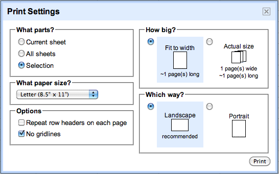
With the power of the cloud, you have access to and can share your files from basically any device without needing to print out anything. We understand that there are occasions when you still need to print, however, and that’s why today we’re happy to announce two new features for printing: selection printing and gridless printing. These two new options allow you to not only customize your printouts, but also save ink in the process.

With selection printing you can print a highlighted section from your spreadsheet. The new option to not print the default gridlines is valuable if you’re trying to print a handout or trying to save ink. You can access these settings via File > Print.


These printing improvements are a direct result of feedback from many of you. If you have more ideas, let us know in the forums.

Posted by: Julian Mcauley, Software Engineering Intern

In-cell dropdown and validation in spreadsheets

Today, we added in-cell dropdown and validation to spreadsheets. This makes it easy to constrain the values of an individual cell to a specific range or list. For example, if you are building a trip planning spreadsheet, you can now limit the options in the travel destination column to a select set of cities via dropdown lists.

In-cell dropdowns also make input easier by reducing unnecessary typing and errors in processing. You can create dropdown lists in individual cells through the data validation tool by validating against a range of cells in your sheet or by creating a custom list.

Follow these steps to create an in-cell dropdown list through validation against a range.

1. Enter data into a range of cells.
• For example, create a list of destinations on your spreadsheet.
2. Select the cell(s) you would like to validate.
3. Under the Tools menu, select Data validation...
4. Change the Criteria to ‘Items from a list.’
5. Click the button next to the ‘Create list from range’ option and select the range of cells you entered data in during Step 1.
   
6. Click Save and the cell you chose to validate will have a dropdown arrow in it with the data in your cell range as the potential input values. If you want, you can set a cell to allow invalid data.

You can also create a in-cell dropdown using a custom list.

1. Under the Tools menu, select Data validation...
2. Change the Criteria to ‘Items from a list.’
3. Click the button next to the 'Enter list items' option.
4. Enter a set of custom values, separated by commas. For example, you could enter "San Francisco, New York, Chicago and Los Angeles."
5. Click Save and the cell you selected will have a dropdown list with the values you entered as potential input values.
   

Let us know what you think in the comments.

Posted by: Li-Wei Lee, Software Engineer

Show all formulas in your spreadsheets

Finding cells that include formulas in them can sometimes be a bit like looking for something in the dark. To help you illuminate your spreadsheet surroundings, we’re introducing the ability to reveal all formulas with one click.

When you’re comparing formulas with one another or trying to figure out where your formulas aren’t working, showing all formulas should help you out. You can turn this feature on from the formula bar by selecting the “Show All Formulas” button, selecting “Show All Formulas” in the View menu or hitting Ctrl `.

Flip the switch in your spreadsheets to try it out.

Posted by: Matt Ziegelbaum, Software Engineer

Check spelling in Google spreadsheets

Correct spelling is an essential part of document creation and today we woild liek to annnounce that spelll chceking is now available in Google spreadsheets.

To launch the new spell checker, go to Tools > Check spelling. The tool will go through all the cells on your sheet, highlighting each cell which has a misspelled word in red. Words that might be misspelled in each cell are underlined in red and can be changed by clicking on them and selecting the right spelling.

Click Next to go to the next cell and once all the cells on one sheet have been checked, you can continue to the next sheet.

The ability to add words to your own dictionary is also coming. You can learn more about the spell checker here. Let us know what you think in the comments.

Posted by: Jonathan Adams, Software Engineering Intern